Dense core collapse with RAMSES
This document is aimed as a tutorial to explore the physics of the protostellar collapse using the RAMSES code. If you have never used RAMSES, you can take a look at the RAMSES fundamentals tutorial. Otherwise you can proceed directly with this tutorial.
Once you have installed RAMSES, in a Terminal, export the proper path to the bin directory, and to the directory where you have downloaded this tutorial:
export RAMSESPATH=/path/to/ramses/bin/
export TUTOPATH=/path/to/this/tutorial/where/you/will/run/the/simulations
You are now ready to begin this tutorial.
Star formation is a complex problem which invokes a huge range of scales, physical processes (MHD, radiation, self-gravity etc.) and components (gas, dust, photons etc.). In this project, we are going to investigate a particular problem of star formation, which is the gravitational collapse of dense cores (or prestellar cores) which occurs when they reach their Jeans mass. This process is at the origin of star formation and also, around the star and through angular momentum conservation, protostellar disk formation.
1. Collapse setup
1.1 Generalities
As often when studying the interstellar medium (ISM), the question of initial conditions is tricky. In the collapse case we should, in principle start from very large scales (arguably galactic scales) and zoom-in up to dense core scales. While some groups are investigating this problem, this is of course not possible for a practical session. Therefore we are going to use a much simple set of initial conditions: the Boss and Bodenheimer setup (Boss & Bodenheimer 1979).
In this setup, we consider an isolated spherical dense core of mass M, radius R and temperature T. Generally, we fix the mass and temperature and compute the radius to ensure that the cloud is gravitationally collapsing. Often, we fix the radius using the thermal-to-gravitational energy ratio \(\alpha\) (or Virial parameter).
\(\alpha = \frac{5}{2} \frac{R}{GM} \frac{k_B T}{\mu_g m_H}\)
where \(G\) and \(k_B\) are the gravitational and Boltzmann constants and \(\mu_g=2.31\) is the mean molecular weight. We usually the fix the simulation box size to be four times the cloud radius.
You can also add some solid body rotation \(\Omega\), assuming a certain value for rotational-to-gravitational energy ratio \(\beta\). To initialize \(\Omega\), we define \(\beta\) such as
\(\beta =\frac{R^3 \Omega^2}{3 \mathcal{G} M_{\odot} }\)
Typically, we set it to a few percent, which is in lines with observations of prestellar cores.
1.2 Equation of state
The radiative transfer during the collapse is, in principle, a quite complex business and requires to use a radiative transfer (RT) solver which is able to treat properly infrared radiation. We often circumvent the issue by assuming a barotropic equation of state (EOS) as follows
\(P = \rho c_{s,0}^2 \left[1 + \left(\frac{\rho}{\rho_{\mathrm{ad}}}\right)^{\gamma-1}\right]\)
This equation allows to recover the two regimes of the first collapse, namely the isothermal phase at low density when radiation can escape freely from the core in the infrared (IR) and the adiabatic contraction of the first Larson core at high density (\(\rho>\rho_{\mathrm{ad}}\simeq 10^{-13} \rm{g/cm}^3\)).
1.3 Parameter file (the namelist)
Here is a summary of the most important parameters that are relevant for collapse calculations. You have to set them in your nml file prior running the simulation. Note that you can find information on all the other namelist parameters you can play with here: https://ramses-organisation.readthedocs.io/en/latest/wiki/Runtime_Parameters.html
RUN_PARAMS. This section defines some of the most basic properties of the run, and the important ones for us here are the following:
hydro=.true.    ! We solve the hydro equations
poisson=.true.  ! We solve the Poisson equation
nrestart=0      ! This not a restart. Set to i (the output i) to restart
nremap=10       ! We do the load balancing every 10 dt. This should be reduced for big runs.
nsubcycle=6*1,2 ! We do sub cycling but not for the 6 first level of refinement (starting from lmin)
AMR_PARAMS. This defines the global mesh properties and memory footprint of the code with the following parameters:
levelmin=5             ! this is the lowest level (same that in the initial conditions).
levelmax=15            ! This is the maximum level of refinement level allowed.
ngridmax=1000000       ! This is the maximum number of grids (oct) that we allow
nexpand=2              ! is the smoothing of the grid at the boundary between levels
boxlen=1.              ! This is the box size in code units (this value should be set carefully, see below)
BOUNDARY_PARAMStells RAMSES what boundary conditions to use. By default, periodic boundaries are used. Here this is zero gradients
nboundary = 6
bound_type= 2, 2, 2, 2, 2, 2
ibound_min=-1,+1,-1,-1,-1,-1
ibound_max=-1,+1,+1,+1,+1,+1
jbound_min= 0, 0,-1,+1,-1,-1
jbound_max= 0, 0,-1,+1,+1,+1
kbound_min= 0, 0, 0, 0,-1,+1
kbound_max= 0, 0, 0, 0,-1,+1
INIT_PARAMStells RAMSES about the initial conditions we want to set.
condinit_kind='collapse' ! Sets the kind of initial collapse
alpha_dense_core=0.35    ! Sets the thermal-to-gravitational ratio (fixing the cloud radius for a given temperature)
beta_dense_core=0.0      ! Sets the amount of rotation
crit_dense_core=0.0      ! Sets the inverse mass-to-flux ratio (the criticality of the core)
delta_rho=0.0            ! Sets the amplitude of the m=2 density perturbation
theta_mag=0.             ! Sets the angle in degrees between the magnetic and rotation axis
OUTPUT_PARAMSdefines the output strategy. Here we make a snapshot evrery 50 dt and also dump the ouptuts of the tout array (times are in code units).
foutput=50
noutput=4
tout=0,1,2,3
POISSON_PARAMSdefines the parameters for gravity
gravity_type=0 ! We solve self-gravity
epsilon=1d-4   ! Tolerance for the error on the gravitational potential
cg_levelmin=7  ! Minimum level from which the Conjugate Gradient solver is used in place of the Multigrid solver
HYDRO_PARAMSdefines the parameters for the hydrodynamics
gamma=1.666667      ! Adiabatic index
courant_factor=0.8  ! Safety factor for the courant conditions, sets the timestep (>1 is unstable)
slope_type=1        ! Slope limiter for the predictor corrector. 1= minmod
scheme='muscl'      ! Scheme to solve the hydro
riemann='llf'       ! Riemann solver. Good options are llf, hll, hllc.
UNIT_PARAMSdefines the constants to be used to convert values from code unit to cgs
units_density= 3.83584509e-24      ! so that density in code units is equal to density in part/cc
units_length= 3.0856776e+18        ! 1 pc in cm
units_time= 1.9769994708456518e15  ! so that G=1 in code units
COOLING_PARAMSdefines the barotropic EOS
barotropic_eos=.true.
barotropic_eos_form='double_polytrope' ! type of barotropic eos
polytrope_rho=1d-13                    ! sets rho_ad in EOS, in g/cm3
polytrope_index=1.666667               ! sets gamma in EOS
T_eos=10d0                             ! sets T0 in EOS, in K
mu_gas=2.31d0                          ! molecular weight
REFINE_PARAMSdefines the refinement strategy. Here we implement a Jeans-length based refinement, where any cell with more than 20 points per Jeans length for 10 successive levels
jeans_refine=20*10. ! Jeans refinement strategy
We provide a barotrop.nml file which will be the basis for this tutorial. This file will need to be adapted to the specific initial conditions you want to use. To do so, we provide below a routine setup_nml which computes the different namelist parameters to be changed accordingly when fixing \(\alpha\), \(M\), \(T\), and the output times.
In all the simulations below, we will use \(\alpha=0.35\), \(M=1\,M_\odot\), \(T=10\,\mathrm{K}\), and \(t_{\rm out}=0.,0.25,0.5,0.75,1,1.25,1.5\) t\(_{\rm ff}\).
[ ]:
import numpy as np

def setup_nml(alpha_dense_core=0.1,mass_c=1.,T_eos=10,tout=(0,1)):
    '''
    alpha_dense_core  : cloud virial parameter, thermal-to-gravitational energy
    mass_c            : cloud mass in solar mass
    T_eos             : cloud temperature

    tout              : output times in free-fall time units
    '''

    # from RAMSES amr/constants.f90 file
    mH=1.6605390e-24      # H atom mass [g] = amu, i.e. atomic mass unit; NIST
    kB=1.3806490e-16      # Boltzmann const. [erg K-1]; SI
    M_sun = 1.9891000e+33 # Solar Mass [g]; IAU

    pc2cm   = 3.0856776e+18  # pc [cm]
    kyr2sec = 3.15576000e+10 # Kyr [s]

    G=6.67e-8 # Gravitational constant in cgs [cm3 g-1 s-2]

    mu_gas=2.31           # Mean molecular weigth

    units_length=pc2cm                      # 1 pc in cm
    units_density=mu_gas*mH                 # so that density in code units is equals to density in part/cc
    units_time=1./np.sqrt(G*units_density)  # so that G=1 in code units

    scale_d = units_density
    scale_t = units_time
    scale_l = units_length
    scale_m=scale_d*scale_l**3

    mass_c_cu = mass_c * (M_sun / scale_m ) # cloud mass in code units

    r0=(alpha_dense_core*2.*G*mass_c_cu*scale_m*mu_gas*mH/(5.*kB*T_eos))/scale_l
    boxlen=4*r0
    d0=3.0*mass_c_cu/(4.0e0*np.pi*r0**3.)

    tff=np.sqrt(3*np.pi/(32*G*d0*scale_d))/scale_t

    print('Cloud size in code units, and in pc=',r0,r0*scale_l/3.0856776e+18)
    print('  box size in code units, and in pc=',boxlen,boxlen*scale_l/3.0856776e+18)
    print('Free-fall time in code units, and in kyr=',tff,tff*scale_t/3.15576000e+10)
    print()
    print('Values to be put in the namelist')
    print('In UNITS_PARAMS')
    print('   units_density=',units_density)
    print('   units_length=',units_length)
    print('   units_time=',units_time)
    print('In AMR_PARAMS')
    print('   boxlen=',boxlen)
    print('In OUTPUT_PARAMS')
    print('   tout=', ', '.join(str(t*tff) for t in tout))
[ ]:
setup_nml()
2. A quick first collapse model : exploration of the first Larson core
2.1 Hydro collapse without rotation
Let’s now run a first collapse calculation with the aim of writing a python pipeline to analyse it.
To perform this analysis we will use the documentation of Osyris (available at https://osyris.readthedocs.io/en/stable/).
To run our calculation we first need to compile the code
cd $RAMSESPATH
make clean
make SOLVER=mhd NDIM=3 MPI=1
You have now a ramses3d executable that can be used to run collapse calculations (using the correct namelist).
Now you will have to copy the executable and the namelist file into the collapse-run directory where you want to run the simulation. Once it’s done you can go in this directory. Let’s assume you want to run the code with 4 CPUs, then the commands are simply
cd $TUTOPATH
mkdir RUN1
cp $RAMSESPATH/ramses3d RUN1
cp barotrop.nml RUN1
cd RUN1
mpirun -np 4 ramses3d barotrop.nml
Note that you can keep the terminal information in a log file (e.g. collapse.log) with the command. To do so, replace the last command by
mpirun -np 4 ramses3d barotrop.nml > collapse.log
Let’s now analyse this first simulation by performing 100 au x 100 au slices in the x,y and z directions. You should have the following results.
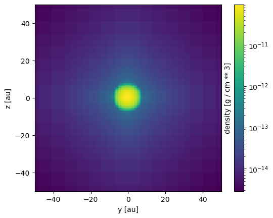
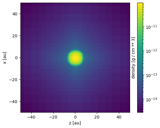
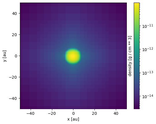
As can be seen in these figures, in this particular case of a collapse without rotation, the first Larson core remains mostly spherical.
[ ]:
import osyris
import numpy as np
au = osyris.units("au")
data = osyris.RamsesDataset(10, path='RUN1').load() # Change this path to the path of the model
# We find the center according to the density
ind = np.argmax(data["mesh"]["density"])
center = data["mesh"]["position"][ind]
osyris.map(
    data["mesh"].layer("density"), norm="log", dx=100 * au, origin=center, direction="x"
)
osyris.map(
    data["mesh"].layer("density"), norm="log", dx=100 * au, origin=center, direction="y"
)
osyris.map(
    data["mesh"].layer("density"), norm="log", dx=100 * au, origin=center, direction="z"
)
2.2 Making movies
The RAMSES simulation namelist contains a block MOVIE_PARAMS (see also the documentation for details), which tells the code to generate binary files with short time intervals showing face-on and edge-on projections of gas density at different zooms.
The first cell below reads those binary files and creates .png images out of them.
The second cell then calls ffmpeg to squeeze all those pngs into one .mp4 movie file. For that second cell to work, you need to have ffmpeg installed.
To download and install ffmpeg, you can use a package manager such as sudo apt install ffmpeg (Ubuntu), brew install ffmpeg (Mac OS), or load it through a module module load ffmpeg (e.g. on a cluster).
As a last resort, you may compile it from source as follows: bash git clone https://git.ffmpeg.org/ffmpeg.git ffmpeg cd ffmpeg ./configure make make install
[ ]:
# Read binary movie frames and make .png images
import os
import glob
import numpy as np
from scipy.io import FortranFile
import matplotlib
import matplotlib.pyplot as plt
from matplotlib.colors import ListedColormap
import matplotlib.patches as mpatches
from tqdm import tqdm

def create_png_for_movie(path='.',movie_number=1):
    if movie_number == 1:
        bar_length_to_be_plot = 1000
    elif movie_number == 2:
        bar_length_to_be_plot = 100
    elif movie_number == 3:
        bar_length_to_be_plot = 100
    else:
        print('Bad value for variable movie_number')

    plt.ioff() # So as not to show plots
    #plt.ion() # So as to show plots
    fig = plt.figure(frameon=False)
    nx = 1920
    ny = 1080
    nypic=ny  #int(ny*0.6)
    plt.subplots_adjust(left=0., bottom=0.,
                    right=1.+1.0/nx, top=1.+1.0/nypic,
                    wspace=0., hspace=0.)
    fig.set_size_inches(nx/100.*.7,nypic/100.*.7)

    #As defined via movie_vars_txt in setup.nml
    quants = {
        "dens": {
            "name": "dens",
            "data": np.array([]),
            "min": 1e6,
            "max": -1e10,
        }
    }

    d_cmap=matplotlib.cm.viridis

    movie_path = '%s/movie%d/'%(path,movie_number)
    png_dir = '%s/pngs'%(path)
    try:
        os.mkdir(png_dir) # Create directory to store movie frames in png files
    except FileExistsError:
        do_nothing=True
    all_ok = True

    # Figure out the number of frames for the movie
    searchstring = '%s/info_'%(movie_path)
    frames = glob.glob(searchstring+'*') # Frame strings
    i_frames = [ int(str[len(searchstring):len(searchstring)+4]) for str in frames ]
    i_frames = sorted(i_frames)         # Sort them
    imin = i_frames[0]
    imax = i_frames[len(i_frames)-1]

    # Loop over the movie frames and generate .png images
    for i in tqdm(range(imin,imax+1)):
        # Read the info file:
        try:
            info = open(f"{movie_path}info_{str(i).zfill(5)}.txt").readlines()
            pass
        except:
            continue
        time_sec=0.0
        time_sec = float(info[8].split("=")[-1].strip())
        unit_l =   float(info[15].split("=")[-1].strip())
        unit_d =   float(info[16].split("=")[-1].strip())
        unit_t =   float(info[17].split("=")[-1].strip())
        time_kyr = time_sec*unit_t/3.156e10

        # Load in the data
        for q in quants:
            fname = f"{quants[q]['name']}_{str(i).zfill(5)}.map"
            ffile = FortranFile(f"{movie_path}{fname}")
            [time, fdw, fdh, fdd] = ffile.read_reals('d')
            [frame_nx, frame_ny] = ffile.read_ints()
            data = np.array(ffile.read_reals('f4'), dtype=np.float64)
            try:
                quants[q]["data"] = data.reshape(frame_nx,frame_ny)
                quants[q]["min"] = quants[q]["data"][quants[q]["data"] > 0].min()
                quants[q]["max"] = quants[q]["data"][quants[q]["data"] > 0].max()
                quants[q]["data"][quants[q]["data"] < quants[q]["min"]] = 1e-5 * quants[q]["min"]
            except ValueError:
                all_ok = False
            f, axs = plt.subplots(1,1,figsize=(7.5,7.5),sharex=True,sharey=True)
        plt.subplots_adjust(left=0, right=1.0, top=1.0, bottom=0)
        axs.imshow(np.log10(quants["dens"]["data"]),vmin=4,vmax=12,cmap=d_cmap,aspect='auto',interpolation='none')
        plt.axis("off")
        # Text showing simulation time
        axs.text(0.97, 0.03,'%.2f kyr'%(time_kyr), fontsize=15,transform=axs.transAxes
             , verticalalignment='bottom', horizontalalignment='right', color='white')
        # Bar showing length scale
        frame_width_au = fdw*unit_l/1.496e+13
        rect = mpatches.Rectangle((0.055,0.03),bar_length_to_be_plot/frame_width_au,0.002,color='white',transform=axs.transAxes)
        axs.add_patch(rect)
        axs.text(0.055, 0.01+15./frame_ny, ('%d au'%(bar_length_to_be_plot)),
            verticalalignment='bottom', horizontalalignment='left',
            transform=axs.transAxes, color='white', fontsize=15. )

        # Store frame in png file
        filename = '%s/frame_%d_%05d.png'%(png_dir,movie_number,i)
        #print(filename)
        f.savefig(filename, dpi=100)
        plt.close()

    return
[ ]:
# Run ffmpeg to make a .mp4 out of the .png frames
import subprocess

def create_mp4_from_png(path='.',movie_number=1):
    movie_filename = '%s/movie%d.mp4'%(path,movie_number)
    frames = '%s/pngs/frame_%d_%%*.png'%(path,movie_number)
    fps=50.
    speed=60.
    quality=23
    print("Calling ffmpeg! Output: {mov}".format(mov=movie_filename))
    print("{binffmpeg} -i {input}\
                     -y -vcodec h264 -pix_fmt yuv420p\
                     -r {fps} -filter:v 'setpts={speed}*PTS'\
                     -crf {quality} {output}".
                    format(binffmpeg='ffmpeg', input=frames,
                           fps=fps, speed=speed/fps,
                           quality=quality, output=movie_filename))
    subprocess.call("{binffmpeg} -i {input}\
                     -y -vcodec h264 -pix_fmt yuv420p\
                     -r {fps} -filter:v 'setpts={speed}*PTS'\
                     -crf {quality} {output}".
                    format(binffmpeg='ffmpeg', input=frames,
                           fps=fps, speed=60./fps,
                           quality=quality, output=movie_filename), shell=True)
    print('####################################################################')
    print('-----------Your new movie is here: ', movie_filename)
    print('####################################################################')

    return
[ ]:
path='RUN1'
movie_number = 2 # movie ID #################### CHANGE THIS FOR THE 3 DIFFERENT MOVIES

create_png_for_movie(path,movie_number)
[ ]:
create_mp4_from_png(path,movie_number)
2.3 More fun
Before you do this analysis, you should start the next simulations which take a longer time to complete.
We can now start to extract structures (such as the first core) to analyse the model. When the density reaches values higher than \(10^{-11}\,\mathrm{g\,cm^{-3}}\), fragments called first Larson cores are forming. We propose to measure the mass as a function of time. This will require to filter the data with masks (using the criterion \(\rho>10^{-11}\,\mathrm{g\, cm^{-3}}\)) and to perform the mass measurement on these filtered data. You can try to play with the initial cloud mass to see if it impacts or not the mass of the First larson core.
3. Adding rotation
Let’s now add rotation to the previous setup (you should run these new simulations in a new directory, e.g. RUN2). The solid body rotation rate is controlled with the beta_dense_core parameter. Typically, you can choose a value between 0.01 and 0.05 to stay in the observed range of dense core (the image of the tutorial is done with 0.05). You should also set delta_rho to 0.1. This sets a m=2 density perturbation of 10% amplitude which prevent the formation of a spurious m=4 mode which could
unfortunately form as a consequence of the cartesian grid.
Let’s now play with this parameter and see its impact on the fragmentation and disk formation during the collapse. For that, we need to push a bit the calculation, as fragmentation will not happen immediately. We will need to run the simulation at least up to output 16 (more ore less a few depending on your choice of initial conditions). If time is limited, we can distribute some outputs to analyse them once you have run the first timesteps yourself.
A 500 au x 500 au slice in the z and y direction obtained with OSYRIS for the snapshot 16 centered at the position of the density maximum should look like this
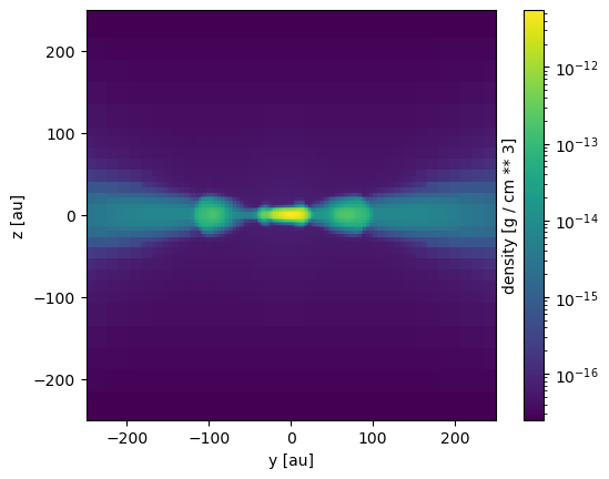
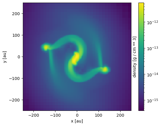
With the z-slice, we clearly see that the core has fragmented into several objects. With the x-slice, it also becomes clear that matter is organised in a thin disk-like rotationally supported structure which is the consequence of angular momentum conservation.
[ ]:
import osyris
import numpy as np
au = osyris.units("au")
data = osyris.RamsesDataset(16, path='RUN2').load() # Change this path to the path of the model
# We find the center according to the density
ind = np.argmax(data["mesh"]["density"])
center = data["mesh"]["position"][ind]
osyris.map(
    data["mesh"].layer("density"), norm="log", dx=500 * au, origin=center, direction="z"
)

osyris.map(
    data["mesh"].layer("density"), norm="log", dx=500 * au, origin=center, direction="x"
)
More fun
We can count the fragment, look at their separation as a function of time and their mass distribution as a function of the rotation rate, the density perturbation. It is also interesting to look at the disk properties, when a disk is formed. For that we need to have some seletion criterion for the disk. Typically, we consider that a disk is a dense and rotationally supported structure. To extract it, we can use the following criterion. The disk material must be
Dense enough.
Supported by rotation
Not thermally supported (this is the first core).
Once you have extracted the disk, try to measure its size and mass as a function of the time. You can also play with the extraction parameters.
The same figure as before but with the disk selection should look like this:

[ ]:
import osyris
import numpy as np
au = osyris.units("au")
data = osyris.RamsesDataset(16, path='./RUN2/').load() # Change this path to the path of the model
# We find the center according to the density
ind = np.argmax(data["mesh"]["density"])
center = data["mesh"]["position"][ind]
condition = (data["mesh"]["density"] < (5.0e-14 * osyris.units("g/cm**3"))) | (
    data["mesh"]["density"] > (5.0e-12 * osyris.units("g/cm**3"))
)
data["mesh"]["disk_density"] = osyris.Array(
    np.ma.masked_where(condition.values, data["mesh"]["density"].values),
    unit=data["mesh"]["density"].unit,
)
osyris.map(data["mesh"].layer("disk_density"), dx=500 * au, norm="log", origin=center,direction='z')
4. Magnetic fields
4.1 Aligned magnetic fields
Dense core are actually magnetised, and the magnetic field, although likely sub-critical is likely to be dynamically relevant. Usually, we set the magnetic field strength according to the mass-to-flux ratio \(\mu\) (in units of critical mass-to-flux ratio): $ \mu`=:nbsphinx-math:frac{left(M/phiright)}{left(M/phiright)_{rm crit}}`$, where \(\phi=\pi B R^2\) and \(\left(M/\phi\right)_{\rm crit}=\frac{0.53}{3\pi}\sqrt{\frac{5}{G}}\) (Mouschovias & Spitzer 1976).
When \(\mu>1\), the collapse can happen, typically \(1<\mu<10\) in dense cores, so let’s explore here this range. By setting the parameter crit_dense_core in the namelist, we are setting \(\frac{1}{\mu}\). We can start to run a simulation with crit_dense_core=0.3, starting from the previous setup (run it in a new directory RUN3). For this value the magnetic field is important while not strong enough to stop the collapse.
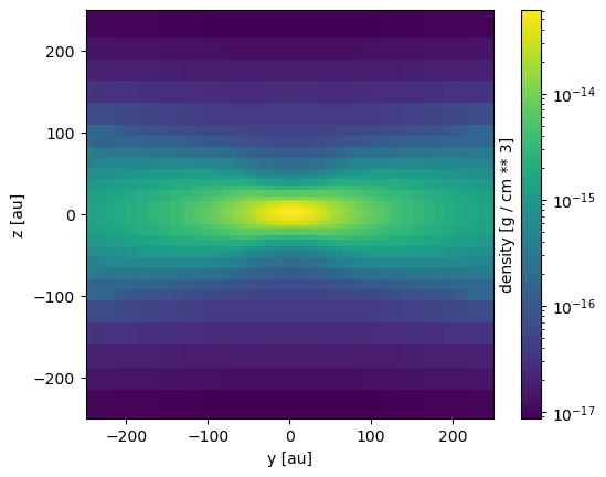
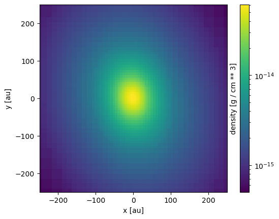
Let’s look again at the collapse seen face-one (z slice). Normally, you should see that for mass-to-flux ratio of the order of a few, the disk is gone. We can observe a dense thin structure around the first core but this is not a disk, this is a pseudo-disk. The pseudo-disk is a consequence of the pinching of the magnetic field line that compress the matter in the equatorial plane but it is not a supported structure (it is collapsing).
Here is a 500 au x 500 au slice in the x direction obtained with OSYRIS that shows the pseudo-disk for a collapse model with crit_dense_core=0.3.
[ ]:
import osyris
import numpy as np
au = osyris.units("au")
data = osyris.RamsesDataset(13, path='./RUN3/').load() # Change this path to the path of the model
# We find the center according to the density
ind = np.argmax(data["mesh"]["density"])
center = data["mesh"]["position"][ind]
osyris.map(
    data["mesh"].layer("density"), norm="log", dx=500 * au, origin=center, direction="z"
)

osyris.map(
    data["mesh"].layer("density"), norm="log", dx=500 * au, origin=center, direction="x"
)
Why is the disk gone ? During the collapse, the twisting of the magnetic field lines generates an intense magnetic braking which suppresses rotation. This so-called magnetic braking catastrophe is a classic problem in the disk formation community. You can take a look at the magnetic field lines to see both the pinching and twisting on the field.
This problem is now solved for the most part by including non-ideal MHD processes that decouple the gas from the magnetic field but are unfortunately not yet implemented in the public version of ramses. Two other potential solutions to recover the disks have also been brought-up by the community: a misalignment between the magnetic field and the rotation axis and turbulence.
Quite interestingly, magnetised models also produce protostellar outflows, you will see them well if you integrate the model up to output 22. This is good since these outflows are observed. You can look at them with edge-one slices and try to see how they depend on the initial magnetic field strength.
A 500 au x 500 au slice in the x direction obtained with OSYRIS that shows a MHD outflow for a collapse model with crit=0.3 as it propagates in the z direction:

[ ]:
import osyris
import numpy as np
au = osyris.units("au")
data = osyris.RamsesDataset(22, path='./RUN3/').load() # Change this path to the path of the model
# We find the center according to the density
ind = np.argmax(data["mesh"]["density"])
center = data["mesh"]["position"][ind]

osyris.map(
        data["mesh"].layer("density", norm="log"),
        data["mesh"].layer("velocity", mode= "vec"), norm="log", dx=500 * au, origin=center, direction="x"
)
4.2 Misaligned magnetic fields
Let us now pay attention to the case when the axis of rotation and of the magnetic field are misaligned. This angle is controlled by the theta_mag parameter in the namelist. We can start with a value of 60 degrees (you should run the simulation in a new directory, e.g. RUN4).
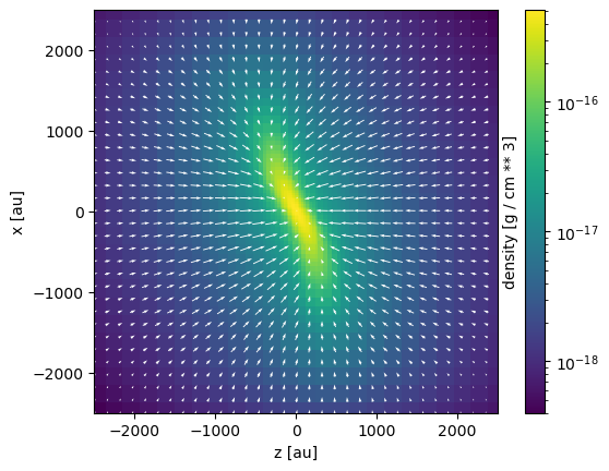
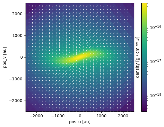
Let’s look at the result early on (output 10) at a relatively large scale. We can see that the flow is tilted with respect to the the z axis because the rotation axis is not z anymore but is tilted by the angle theta_mag.
A 5000 au x 5000 au slice in the y direction obtained with OSYRIS (left panel) shows that the axis of rotation is now tilted by 60 degrees. We can redo the same figure, but making it perpendicular to the new rotation axis thanks to the functionality of osyris which can find the angular momentum axis (right panel).
[ ]:
import osyris
import numpy as np
au = osyris.units("au")
data = osyris.RamsesDataset(7, path='./RUN4/').load() # Change this path to the path of the model
# We find the center according to the density
ind = np.argmax(data["mesh"]["density"])
center = data["mesh"]["position"][ind]

osyris.map(
        data["mesh"].layer("density",norm="log"),
        data["mesh"].layer("velocity",mode="vec"), norm="log", dx=5000 * au, origin=center, direction='y'
    #,filename='run4_slice_y.png'
)

osyris.map(
        data["mesh"].layer("density",norm="log"),
        data["mesh"].layer("velocity",mode="vec"), norm="log", dx=5000 * au, origin=center, direction='top'
    #,filename='run4_slice_top.png'
)
If we now wait a bit longer, and make a ‘top’ slice i.e. a slice in the rotation plane we can see that we now recover a disk.
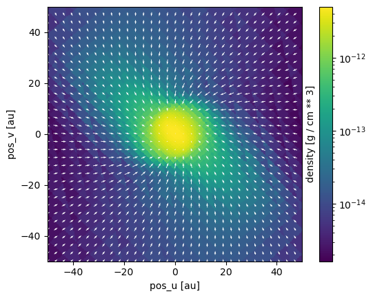

We can play the same game as before (measuring its properties) and also test the disk properties as a function of the angle between the magnetic field and rotation. An interesting question might be: which is the limit angle to form a disk for a given magnetic field strenght?
[ ]:
import osyris
import numpy as np
au = osyris.units("au")
data = osyris.RamsesDataset(18, path='./RUN4/').load() # Change this path to the path of the model
# We find the center according to the density
ind = np.argmax(data["mesh"]["density"])

center = data["mesh"]["position"][ind]

osyris.map(
        data["mesh"].layer("density",norm="log"),
        data["mesh"].layer("velocity",mode="vec"), norm="log", dx=100 * au, origin=center, direction='top'
    #,filename='run4_slice_top_longer.png'
)
[ ]:
import osyris
import numpy as np
au = osyris.units("au")
data = osyris.RamsesDataset(18, path='./RUN4/').load() # Change this path to the path of the model
# We find the center according to the density
ind = np.argmax(data["mesh"]["density"])

center = data["mesh"]["position"][ind]
condition = (data["mesh"]["density"] < (5.0e-14 * osyris.units("g/cm**3"))) | (
    data["mesh"]["density"] > (5.0e-12 * osyris.units("g/cm**3"))
)
data["mesh"]["disk_density"] = osyris.Array(
    np.ma.masked_where(condition.values, data["mesh"]["density"].values),
    unit=data["mesh"]["density"].unit,
)
osyris.map(data["mesh"].layer("disk_density"), dx=100 * au, norm="log", origin=center, direction='z')
5. Initial turbulence
In order to take into account the interstellar turbulence in the initial conditions, another parameter can be used. The Mach parameter in the INIT_PARAMS block of the namelist sets the initial Mach number of a turbulent initial velocity field, which is added to the one set up by beta_dense_core if specified.
You can play around with this parameter to see its influence. In particular, you can see that with a high value of Mach the turbulent support can prevent the collapse.
Note that to do so, you will need a file init_turb.data which contains the initial turbulent velocity field. To generate such a file, you can use the script below, where you will have to specify 3 random number seeds and the value of the power-law index. (Note that if not done yet, you will have to install the turbustat package)
[ ]:
%pip install turbustat
[ ]:
from turbustat.simulator import make_3dfield
from matplotlib import pyplot as plt

# choose random number seeds
# choose powerlaw index
# empirically Gaussian fluctuations power law (modelled by the fBm) is about 3.4 - 3.6 (J.-F. Robitaille)

def generate_init_turb(seed1=824329,seed2=129862,seed3=786276,powerlaw=3.5):
    # choose name for output file
    filename = 'ramses_{}-{}-{}.data'.format(seed1, seed2, seed3)

    # generate fields for the three components of the velocity
    cells=100
    vx = make_3dfield(cells, powerlaw=powerlaw, randomseed=seed1)
    vy = make_3dfield(cells, powerlaw=powerlaw, randomseed=seed2)
    vz = make_3dfield(cells, powerlaw=powerlaw, randomseed=seed3)
    # make plots to verify the fields look OK
    for seed, v in zip([seed1, seed2, seed3], [vx,vy,vz]):
        fig, ax = plt.subplots(nrows=1, ncols=3, figsize=[10, 3])
        ax[0].imshow(v.mean(0), origin='lower')
        ax[1].imshow(v.mean(1), origin='lower')
        ax[2].imshow(v.mean(2), origin='lower')
        plt.tight_layout()
        plt.savefig('seed{}_pl{}.png'.format(seed, powerlaw))
        plt.close()

    # write fields to ramses readable ascii file
    f = open(filename, 'w')
    f.write('{:8}{:13.5f}{:13.5f}{:13.5f}{:13.5f}\n'.format(cells, powerlaw, seed1, seed2, seed3))
    for x in range(cells):
        for y in range(cells):
            for z in range(cells):
                f.write('{:13.5f}{:13.5f}{:13.5f}{:13.5f}{:13.5f}{:13.5f}\n'.format(x, y, z, vx[x,y,z], vy[x,y,z], vz[x,y,z]))
    f.close()
    print('\033[92m' + 'Initial turbulent field ' + filename + ' generated\033[0m')

    return
[ ]:
generate_init_turb()
Once done, then simply rename the generated file to init_turb.data and copy it into the directory where you will run the simulations (e.g. RUN5).
cp ramses_824329-129862-786276.data RUN5/init_turb.data
A non exhaustive list of collapse papers with RAMSES
If you want to dig deeper in the collapses with RAMSES, here is a list of some (but biased and not at all exhaustive) of the papers that were written using this setup (generally with a modified version including more physics):
Hennebelle and Fromang 2008: Magnetic processes in a collapsing dense core I.
Hennebelle and Teyssier 2008: Magnetic processes in a collapsing dense core II.
Commerçon et al. 2010: Protostellar collapse: radiative and magnetic feedbacks on small-scale fragmentation
González et al. 2015: Multigroup radiation hydrodynamics with flux-limited diffusion and adaptive mesh refinement
Vaytet et al. 2018: Protostellar birth with ambipolar and ohmic diffusion
Hennebelle et al. 2020: What determines the formation and characteristics of protoplanetary discs?
Lebreuilly et al. 2020: Protostellar collapse: the conditions to form dust-rich protoplanetary disks
Mignon-Risse et al. 2021: Collapse of turbulent massive cores with ambipolar diffusion and hybrid radiative transfer. I. Accretion and multiplicity
Mignon-Risse et al. 2021: Collapse of turbulent massive cores with ambipolar diffusion and hybrid radiative transfer. II. Outflows
Hennebelle et al. 2022: Influence of magnetic field and stellar radiative feedback on the collapse and the stellar mass spectrum of a massive star-forming clump
Commerçon et al. 2022: Discs and outflows in the early phases of massive star formation: Influence of magnetic fields and ambipolar diffusion
Lebreuilly et al. 2024: Synthetic populations of protoplanetary disks: Impact of magnetic fields and radiative transfer
Commerçon et al. 2024: Discs are born eccentric